The Engineering Behind a RAG (Retrieval-Augmented Generation)

Part 1 of 2 ,Ingestion, Retrieval, and Generation (Done Right)

Most RAG tutorials show you how to build something that works in a notebook.
This one shows you how to build something that works when a real user asks a real question under load, in multiple languages, against messy real-world documents.

I've seen a lot of RAG implementations. The majority share the same failure pattern: the retrieval looks clean in demos, then degrades silently in production. Context windows fill with irrelevant chunks, the LLM hallucinates with alarming confidence, and the team spends weeks tuning prompts instead of fixing the actual plumbing.

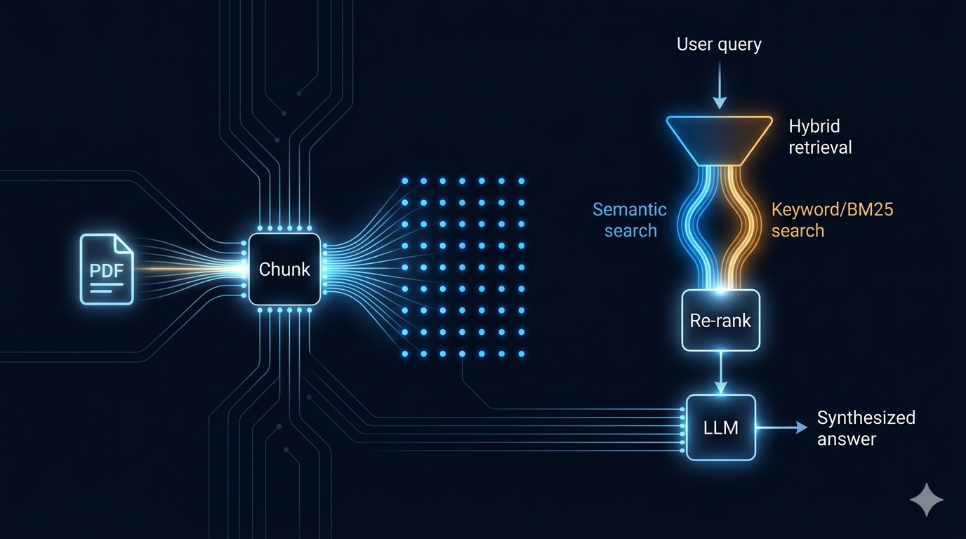
RAG is deceptively simple on the surface: retrieve relevant context, pass it to an LLM, generate an answer. The depth is in the details between those three steps. Let me walk you through what a production-grade pipeline actually looks like — end to end.

The Two Jobs RAG Has

Before anything else, I want to establish the mental model:

RAG = Storing + Retrieving

Everything else — chunking, embeddings, reranking, query rewriting — is in service of one of these two phases. If you keep that split in mind, you'll make better engineering decisions. Every optimization can be categorized: does it improve what we store, or how we retrieve?

Phase 1: Ingestion — What You Store Determines What You Can Find

Source Extraction: The Part Everyone Underestimates

Your pipeline is only as good as the text it operates on. Before you write a single line of embedding logic, ask: what does the text actually look like after extraction?

PDF Ingestion (OCR only when needed)
Not all PDFs are equal. A text-based PDF (most legal docs, reports) can be extracted with pdfminer or PyMuPDF at near-zero cost. An image-based or scanned PDF requires OCR — typically Tesseract or PaddleOCR for multilingual documents. Applying OCR universally is wasteful and introduces unnecessary noise. The right approach:

import fitz  # PyMuPDF
 
def is_text_pdf(path: str) -> bool:
    doc = fitz.open(path)
    text = "".join(page.get_text() for page in doc)
    return len(text.strip()) > 100  # heuristic: if there's text, skip OCR

** Layout-Aware Extraction:** This is the most underrated step in the entire pipeline. Standard text extractors ignore document structure — they treat a two-column academic paper the same as a linear blog post. Layout-aware extractors (like unstructured.io or LayoutParser) understand that a table header belongs to its rows, that a caption belongs to its figure, that a heading contextualizes what follows it. Losing this structure silently destroys retrieval accuracy. A chunk that starts mid-sentence in column 2 of a PDF is nearly unretrievable.

Multilingual documents add another layer. For Arabic, Urdu, or other RTL languages, your extraction library must handle bidirectional text correctly. pdfminer.six with explicit codec handling is far more reliable here than naive PyPDF2.

Web scraping has its own flavour: strip boilerplate (nav, footer, ads) before ingestion. trafilatura does this well and works across languages.

Chunking: The Decision That Echoes Through Everything

Chunking is where most pipelines lose information before retrieval even runs.

There are three chunking strategies worth understanding:

1. Fixed-Size Chunking
Split every N tokens, with M token overlap. Simple, predictable, fast. The problem: it splits sentences, severs context, and has no awareness of semantic boundaries.

def fixed_chunk(text: str, size: int = 512, overlap: int = 64) -> list[str]:
    tokens = text.split()
    chunks = []
    for i in range(0, len(tokens), size - overlap):
        chunks.append(" ".join(tokens[i:i + size]))
    return chunks

Reasonable default. Not good enough for production.

2. Semantic Chunking
Split on sentence boundaries, then group semantically similar sentences together. Uses embedding similarity between adjacent sentences to decide where chunks should break. Result: chunks that hold a single coherent idea. More expensive at ingestion time. Worth it.

3. Hierarchical / Parent-Child Chunking (recommended for complex documents)
Store two chunk sizes: small chunks (for precise retrieval) and large parent chunks (for rich LLM context). Retrieve by small chunk, return the parent. This is the pattern used in LlamaIndex's ParentDocumentRetriever and in production at several enterprise RAG deployments.

Document
├── Parent Chunk (512 tokens) ← passed to LLM
│   ├── Child Chunk A (128 tokens) ← retrieved
│   └── Child Chunk B (128 tokens) ← retrieved

Aside: For multilingual systems, chunking strategy needs to account for language morphology. Arabic and Turkish are morphologically rich — a single word encodes what English expresses in five. Sentence-aware chunking with spaCy or stanza multilingual models preserves semantic integrity far better than token-count splitting in these languages. BGE-M3's own paper empirically validates sentence-aware chunking as optimal for Arabic RAG pipelines.

With overlap, always. 10–15% overlap prevents the edge case where a critical sentence spans a chunk boundary.

Embeddings: The Bridge Between Language and Mathematics

This is where language becomes geometry. A good embedding model maps semantically similar text to nearby points in vector space. A bad one makes your retrieval look random.

Model Selection

| Use Case | Recommended Model | Dimensions | Notes | |---|---|---|---| | English only | text-embedding-3-small (OpenAI) | 1536 | Strong general-purpose | | Multilingual (open) | BAAI/bge-m3 | 1024 | Supports 100+ languages, dense + sparse + multi-vector | | Multilingual (hosted) | voyage-3 | 1024 | Top MTEB scores across languages | | Long documents | nomic-embed-text-v1.5 | 768 | Matryoshka dims, 8k token context |

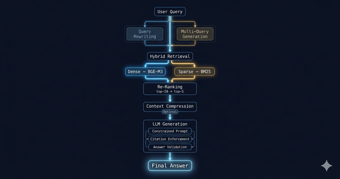
BGE-M3 deserves a special mention for multilingual RAG. It produces three types of representations from one model: dense vectors (semantic), sparse vectors (lexical weight), and multi-vector representations (colBERT-style). This directly enables hybrid retrieval without maintaining separate models.

from FlagEmbedding import BGEM3FlagModel
 
model = BGEM3FlagModel('BAAI/bge-m3', use_fp16=True)
 
# Returns dense, sparse, and colbert vectors simultaneously
output = model.encode(
    chunks,
    batch_size=32,
    max_length=512,
    return_dense=True,
    return_sparse=True,
    return_colbert_vecs=False  # set True for very high accuracy use cases
)
 
dense_embeddings = output['dense_vecs']
sparse_weights = output['lexical_weights']

Tradeoff: Higher embedding dimensions = more storage, slower search. Matryoshka embeddings (Nomic, OpenAI v3) let you truncate dimensions at query time — a powerful cost lever. At 256 dimensions they're 6× faster to search with minimal quality loss for most retrieval tasks.

What actually happens inside an embedding model:

Text → Tokenizer (vocab-specific BPE/WordPiece) 
     → Token IDs 
     → Transformer encoder (12–24 layers of attention) 
     → [CLS] token representation 
     → L2-normalized vector ∈ ℝᵈ

The model is not "summarizing" — it's projecting language into a geometric space where cosine distance approximates semantic distance. That distinction matters when you debug retrieval failures.

Phase 2: Retrieval — What You Find Determines What the LLM Can Say

Dense Retrieval (Semantic Search)

The baseline: embed the query, find the nearest stored vectors. Fast, powerful, language-agnostic. But it fails on:

Exact keyword requirements ("what does Article 7 say")
Proper nouns, product names, version numbers
Short or underspecified queries

query_embedding = model.encode("eligibility criteria")['dense_vecs']
results = qdrant_client.search(
    collection_name="docs",
    query_vector=query_embedding,
    limit=20
)

Sparse Retrieval (BM25 / Keyword Matching)

BM25 is a probabilistic keyword scoring function. Decades old, still best-in-class for exact lexical matching. It fails where dense retrieval succeeds: long, nuanced semantic queries.

The insight: they fail in complementary ways. This is why you combine them.

Hybrid Retrieval — The Production Default

score = α × semantic_score + (1 - α) × bm25_score

The alpha weight is tunable per domain. Legal documents: higher BM25 weight (precision matters). Customer support: higher semantic weight (paraphrase tolerance matters).

Reciprocal Rank Fusion (RRF) is an alternative that doesn't require score normalization across systems:

def rrf_score(rank: int, k: int = 60) -> float:
    return 1.0 / (k + rank)
 
# Merge results from dense and sparse retrievers
combined = {}
for rank, result in enumerate(dense_results):
    combined[result.id] = combined.get(result.id, 0) + rrf_score(rank)
 
for rank, result in enumerate(bm25_results):
    combined[result.id] = combined.get(result.id, 0) + rrf_score(rank)
 
final = sorted(combined.items(), key=lambda x: x[1], reverse=True)

Qdrant's native hybrid search handles this at the infrastructure level. Milvus and Weaviate have similar primitives.

Aside for multilingual systems: BM25 requires language-aware tokenization to work correctly. A BM25 over Arabic text needs a proper Arabic morphological analyzer (e.g., CAMeL Tools), not a naive whitespace tokenizer. BGE-M3's sparse output is a stronger choice in multilingual contexts because it produces learned lexical weights rather than raw term frequencies.

Query Rewriting — Bridging the User-Document Gap

Users ask bad questions. Not because they're unintelligent, but because they're thinking in conversation, not in information retrieval.

"what about the penalty?" — penalty for what? In which document? In which context?

Query rewriting uses an LLM to transform the raw user query into a form that better matches the language of stored documents:

REWRITE_PROMPT = """
Given the user query and conversation history, rewrite the query to be:
- Self-contained (not dependent on context)
- Specific (include domain/subject)
- Optimized for document retrieval
 
Conversation history: {history}
User query: {query}
 
Rewritten query:
"""

Tradeoff: Query rewriting adds 100–300ms latency and one LLM call per query. For conversational systems where queries are ambiguous and follow-ups are common, the retrieval quality gain is worth it. For single-turn fact lookup systems, skip it.

Multi-Query Retrieval — Covering the Semantic Surface

A single query hits one point in embedding space. For complex questions, that's not enough coverage.

Generate 3–5 query variations, retrieve for each, deduplicate by chunk ID:

MULTI_QUERY_PROMPT = """
Generate 4 variations of the following query that ask for the same information
from different angles. Return as a JSON array.
 
Query: {query}
"""
 
# Retrieve for each variation, deduplicate
all_chunks = {}
for variation in generated_queries:
    results = retrieve(variation)
    for chunk in results:
        all_chunks[chunk.id] = chunk  # dedup by ID
 
final_candidates = list(all_chunks.values())

Aside: This is particularly powerful for multilingual systems. You can generate query variations in multiple languages and retrieve across language boundaries — critical if your document corpus is multilingual but queries come in primarily one language.

Re-Ranking — The Step That Earns Its Cost

Vector similarity is cheap to compute but semantically imprecise. A cross-encoder re-ranker takes the top-20 retrieved candidates and scores each query + chunk pair together — the way a human would evaluate relevance.

Vector DB → Top 20 chunks (approximate similarity)
             ↓
       Cross-Encoder Re-ranker
             ↓
         Top 5 chunks (actual relevance)
             ↓
            LLM

from sentence_transformers import CrossEncoder
 
reranker = CrossEncoder('cross-encoder/ms-marco-MiniLM-L-6-v2')
 
# For multilingual: use 'BAAI/bge-reranker-v2-m3'
reranker_ml = CrossEncoder('BAAI/bge-reranker-v2-m3')
 
pairs = [(query, chunk.text) for chunk in candidates]
scores = reranker.predict(pairs)
 
ranked = sorted(zip(candidates, scores), key=lambda x: x[1], reverse=True)
top_k = [chunk for chunk, _ in ranked[:5]]

Cross-Encoder vs. Bi-Encoder: A bi-encoder (like BGE-M3) embeds query and document independently — fast, scalable, used at retrieval time. A cross-encoder takes query and document as a joint input, enabling full attention across both — slower, far more accurate, used at re-ranking time. This two-stage architecture is the canonical solution to the speed-accuracy tradeoff in information retrieval.

Without re-ranking, your LLM receives the top-20 chunks most similar to the query in embedding space. Several of those will be topically adjacent but not actually relevant. The LLM will hallucinate to fill the gaps between them.

With re-ranking, it receives the 5 chunks most relevant to the specific question asked. The difference in answer quality is measurable and significant.

Phase 3: Generation — Where Hallucination Lives

Retrieval finds the right context. Generation is where the LLM can still go wrong with it.

Context Compression

You've retrieved 5 ranked chunks. But some of those chunks contain only one paragraph relevant to the query, surrounded by noise. Send the whole chunk to the LLM and the noise becomes a distraction.

LLMChainExtractor in LangChain runs a secondary compression step — a lighter LLM pass that strips each chunk to just the sentences relevant to the query before passing to the primary LLM. Use it when precision matters more than latency.

Prompt Constraints — Grounding the LLM

The system prompt is your last line of defense against hallucination:

You are a precise document-answering assistant.

Rules:
1. Answer ONLY using information found in the provided context.
2. If the answer is not in the context, respond: "This information is not available in the provided documents."
3. Do not combine information across chunks unless explicitly connected.
4. Reference the relevant source for each claim.

Context:
{compressed_context}

Question: {query}

This is not a minor formatting detail. The explicit constraint against reasoning beyond the context is the single most effective anti-hallucination measure available without model fine-tuning.

Top-K Tuning

k too high → noisy context → hallucination
k too low  → missing information → incomplete answers

The sweet spot is typically 3–7 final chunks after re-ranking, but it depends on:

Average chunk size (smaller chunks → higher k)
LLM context window (larger window → tolerate higher k)
Domain complexity (multi-faceted questions → higher k)

Run offline evaluations against a golden test set to tune this per domain.

Citation Enforcement

Force the model to cite its sources. This serves two purposes: it keeps the LLM grounded in retrieved text, and it makes hallucinations auditable.

CITATION_PROMPT = """
Answer the question. For each claim, cite the chunk number it comes from.
Format: "claim [chunk_N]"
 
Chunks:
[1] {chunk_1}
[2] {chunk_2}
[3] {chunk_3}
 
Question: {query}
"""

Answer Validation Loop (for high-stakes systems)

Generate an answer, then run a secondary LLM call that verifies each factual claim in the answer against the retrieved chunks. Flag unverified claims for review or rejection.

Generate Answer → Extract Claims → Verify Each Claim Against Chunks
                                         ↓
                              Verified → Return
                              Unverified → Flag / Regenerate

This adds cost and latency, but for domains like legal, medical, or financial applications, the tradeoff is justified.